
Analysis towards the EU ETS markets and related commodities, Coding and Simulation Part: Pricing and Prediction based on equilibrium Fuel Switching Price
import numpy as np
import pandas as pd
import matplotlib.pyplot as plt
The Problem
We assume the price of EU ETS is a martingale. The penalty of incompliance is $\pi$. We have the following: \(A^*_t = \pi E((\Gamma - \Pi(\xi^*))^+ | F_t)\) $\Gamma$ is the total incompliance amount of carbon emission if burning coal. Where $\Pi(\xi)^+$ is the abatement of carbon emission under the abatement strategy $\xi^*$.
Strategy of Abatement
The problem left to find the optimal strategy $\xi$. \(G(\xi) = - \sum\limits^{N}_{i = 1} \sum\limits^{T-1}_{t=0} \xi^i_t \epsilon^i_t - \pi(\Gamma - \Pi(\xi^*))\) \(\xi^* = arg sup E(G)\) Where $\epsilon^i_t$ is the Marginal Abatement Cost. (to decrease unit amount of CO2, how much it costs by switching to another fuel).
By the martingality of allowance price, we are aware: \(E(G|F_t) = E(- \sum\limits^{N}_{i = 1} \sum\limits^{T-1}_{t=0} \xi^i_t \epsilon^i_t - \pi(\Gamma - \Pi(\xi^*)) |F_t) = E(- \sum\limits^{N}_{i = 1} \sum\limits^{T-1}_{t=0} \xi^i_t \epsilon^i_t |F_t) - A^*_t\)
Hence, our strategy could be simplified to switch to coal if $\epsilon_t > A^_t$ and use gas if $\epsilon_t \leq A^_t$
Algorithm
- Initialize the model with the current information $F_t$. Construct two process based on the information we have, that is the fuel switching process and the demand process.
- Then find the $A^*_{t+1}$. Could try to iterate for $M$ times to find the convergency.
- For next time stage, we use the price $A^*{t+2}$ by $F{t+1}$ from step 2
class plant:
    coal_e = 0.36
    coal_emit = 0.26
    gas_e = 0.45
    gas_emit = 0.14
    time_grid = 10
    abatement_requirement = 0.8 #Required to decrease 20% of the total carbon emission
    def __init__(self, T, fs_price, total_demand):
        self.demand = np.zeros(T)
        self.fs_price = np.zeros(T)
        self.fs_price[0] = fs_price
        self.demand_process(total_demand)
        self.T = T
        self.total_allowance = sum(self.demand[:])*self.abatement_requirement*self.coal_emit/self.coal_e
        self.abate = np.zeros(T)

    def update_abate(self, A, t_0):
        #update abatement strategy based on the allowance price A
        for t in range(t_0, self.T):
            if A > self.fs_price[t]:
                #choose gas
                self.abate[t] = self.demand[t]*(self.coal_emit/self.coal_e - self.gas_emit/self.gas_e) #unit in GJ

    def demand_process(self, total_demand):
        #Construct demand process for each day in the period of T
        avg_demand = total_demand/(len(self.demand))
        for i in range(len(self.demand)-1):
            self.demand[i] = avg_demand*(1 + max(-1, 0.3*np.random.normal()))
        self.demand[-1] = max(0,total_demand - sum(self.demand[:-1]))

    def fs_process(self, drift, vol):
        #Construct the fuel switching process. We use log-normal distribution but could be changed to ARMA process.
        for i in range(self.T-1):
            last = self.fs_price[i]
            for j in range(self.time_grid):
                last += (last*drift*1/self.time_grid + last*vol*np.random.normal()*np.sqrt(1/self.time_grid))
            self.fs_price[i+1] = last

    def exceeded_allowance(self, t):
        #Find how much allowance we left or outstanding
        return (sum(self.demand[t:])*(1-self.abatement_requirement)*self.coal_emit/self.coal_e - sum(self.abate[t:]))

    '''
    @staticmethod
    #Could use staticmethod if we want to fix a fs_process for all the agents
    def fs_process(self, drift, vol):
        #Construct the fuel switching process. We use log-normal distribution but could be changed to ARMA process.
        for i in range(self.T-1):
            last = self.fs_price[i]
            for j in range(self.time_grid):
                last += (last*drift*1/self.time_grid + last*vol*np.random.normal()*np.sqrt(1/self.time_grid))
            self.fs_price[i+1] = last
    '''
def test(T, A, M, N, fs_price_0, total_demand, drift, vol, penalty):
    allowance = []
    agents = []
    for i in range(N):
        agents.append(plant(T, fs_price_0, total_demand[i]))
        agents[i].fs_process(drift[i], vol[i])
        agents[i].update_abate(A, 0)
    A = incompliance_p(agents, 0)*penalty
    for h in range(M):
        #iterate M times
        for i in range(N):
            #consider N agents
            agents[i].update_abate(A, 0)
        A = incompliance_p(agents, 0)*penalty
    allowance.append(A)
    for j in range(1,T):
        #from time = 1 to T
        for h in range(M):
            #iterate M times to find the equilibrium
            for i in range(N):
                #consider N agents with different demand process and different fuel switching price due to efficiency
                agents[i].update_abate(A, j)
            A = incompliance_p(agents, j)*penalty
        allowance.append(A)
    return (allowance, agents)
def incompliance_p(agents, t):
    num = 0
    for i in range(len(agents)):
        if(agents[i].exceeded_allowance(t) > 0):
            num += 1
    return num/len(agents)
T = 100
#T days to the end of compliance period
fs_price_0 = 20
#Initial Fuel Switching Price
N = 500
#500 agents
M = 10
#Iterate 10 times for each time t
total_demand = np.zeros(N)
for i in range(N):
    total_demand[i] = 1000
#Total Demand is 1000 mWh for each agent
drift = np.zeros(N)
drift += 0.03
vol = np.zeros(N)
vol += 0.2
penalty = 40
#Penalty
A_0 = 22
#Initial Allowance price
t_0 = 0
(a_l, agents) = test(T, A_0, M, N, fs_price_0, total_demand, drift, vol, penalty)
Attempt
This is a very easy example: We fix the volatility for the fuel switching process as 0.2 (daily), and daily drift as 0.03. The penalty is set as 40/(t CO2). The intial allowance price is set as 22, and the fuel switching price is set as 20 initially.
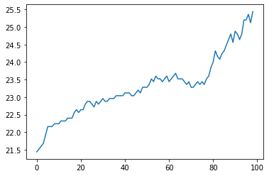
plt.plot(a_l[:-1])
[<matplotlib.lines.Line2D at 0x7f24e3dddc70>]
return_a_l = []
for i in range(len(a_l)-2):
    return_a_l.append(a_l[i+1] - a_l[i])
plt.plot(return_a_l)
[<matplotlib.lines.Line2D at 0x7f24e3dede50>]
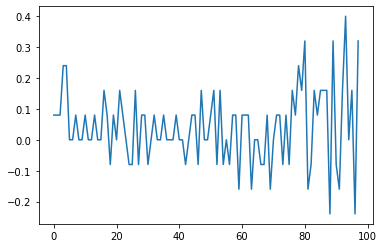
This is the price eastimated allowance price and returns. We could witness as we approach the end of compliance, the price climbs more steep.
for i in range(len(agents)):
    plt.plot(agents[i].abate[:-1])
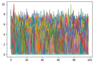
This is the strategy $\xi$ of 500 agent, which is how much CO2 he abates at each time. For example, the following agent decided to abate the CO2 from to time.
agents[11].abate
array([2.4719671 , 2.15194003, 3.84656584, 4.53316987, 3.75449053,
       3.53648264, 0.        , 0.        , 0.        , 0.        ,
       0.        , 0.        , 0.        , 0.        , 0.        ,
       0.        , 0.        , 0.        , 0.        , 0.        ,
       0.        , 0.        , 0.        , 0.        , 0.        ,
       0.        , 0.        , 0.        , 5.86611946, 4.15584676,
       4.06762754, 5.86179706, 0.        , 2.6846712 , 0.        ,
       0.        , 2.50898656, 3.33230104, 4.22091453, 6.76531065,
       3.02182513, 5.18674288, 6.88471192, 5.63564736, 6.21166597,
       5.71933266, 5.09822952, 6.52768913, 4.67036084, 4.7740932 ,
       5.33072482, 2.3107941 , 2.93937432, 3.48477047, 3.74550835,
       6.4358942 , 3.11376885, 4.53686207, 3.15481516, 6.74954726,
       3.77453499, 3.93407629, 4.7240192 , 1.32756929, 4.04351253,
       4.78306741, 4.57095511, 7.5496401 , 6.2271449 , 3.95327001,
       3.44694973, 5.07781318, 4.69536299, 2.62293579, 4.68475071,
       2.99401237, 3.09222157, 3.83504218, 2.42862809, 2.20403407,
       3.20955203, 4.16561558, 0.        , 0.        , 0.        ,
       0.        , 0.        , 0.        , 0.        , 0.        ,
       0.        , 0.        , 0.        , 0.        , 0.        ,
       0.        , 0.        , 0.        , 0.        , 0.        ])
Reflections
Our methods have two strengths compared to statistical methods:
- We just require to initialize the data, and the prediction should have correct dynamics even for long term prediction. (good extensibility)
- We only need to simulate the Fuel Switching Process (one process instead of gas price and coal price process as well)
Some points to be Mentioned:
- If we care about system’s PnL, the change of emission allowance positions between the agents wouldn’t impact the total PnL. (this simplifies the model)
- We consider a fractionless and 0 interest rate model.
The model could be better improved and more close to reality if we:
- Fine tune the generated Fuel Switching Process
- The strategy has to have time gap with the Fuel Switching Process. And we have to be aware it may not fully switch to another fuel, but could be x% for gas and 1-x% for coal (non-linear feature).
Codes
Codes are availble to download from my repository.