Correlation Analysis and Strategy Insights

Fuel Switching Price

To ease the understanding, we choose an easier definition for the fuel switching price. \(\begin{aligned} P_{G} &= \frac{\eta^E_C G - \eta^I_G C}{\eta_G^I e_C^E - \eta^E_C e_G^I} \\ P_{C} &= \frac{\eta^I_C G - \eta^E_G C}{\eta_G^E e_C^I - \eta^I_C e_G^E}\\ \end{aligned}\) Here, $P_G$ means that if the allowance price is higher than $P_G$, we have to switch to Natural Gas. Suppose our allowance price is lower than $P_C$, then we choose Coal. $\eta^E_G, \eta^I_G, \eta^E_C, \eta^I_C$ simply mean the thermal efficiency of an efficient (E) or inefficient (I) plant for Gas (G) and Coal (C). $e^E_G, e^I_G, e^E_C, e^I_C$ is how much carbon burning Coal (C) or Gas (G) an efficient (E) or inefficient (I) plant emit.

The intuition to derive the formulas are very easy. Just find two break even points where an inefficient plant would spend fewer money if he uses natural gas than an efficient plant who relies on coal. And when an efficient coal based plant would spend more money compared to an inefficient natural gas company.

{width=”6cm”}

{width=”6cm”}

Problems of the Correlation

Based on the differenced price of XA1 and TTD1, we first do a window shift of ranging from 30 to 90 to check the correlation between commodities and allowance price.

{#fig:my_label width=”70%”}

The problem with this figure is:

• It is logically incorrect that we always have positive correlation with the return of any one of the two commodities with allowance. - It’s hard to understand why the move of the natural gas is positively correlated with the price of allowance.

  • First of all, suppose the price of natural gas going up, we would anticipate the price of allowance decrease instead of positive correlation.

  • In addition, it is also problematic that there is no time lag - It is very hard for the plants to directly change to another fuel once there is some change to the price.

  • Therefore, my understanding is such positive correlation just reflects the co-movements in the energy market, instead of the correlation from the mechanism of switching the fuel.

• The correlation is higher at the end. This is due to the reason that the price and returns are higher at the end, and they takes up higher weight when measuring correlation.

Adjustments to the correlation measurement

I did two adjustment:

• Use "1", "-1" to measure the increase and decrease instead of the true returns. This could avoid the impact of the magnitude of the moves towards the correlation.

• Test a time lag from $n = 0, 1 ,2, 3, 7, 30$. This means, we are comparing the returns / moves of the fuels with the returns of the allowance after the time shift $n$. For example, a time lag $n = 2$ means we are considering how do the changes to price two days ago in the fuels would affect the allowance price (after the two days).

{width=”6cm”}

{width=”6cm”}

From the correlation with XA1 and TTD1, we could witness our correlation are sometimes positively correlated and negatively correlated. Then we proceed to in-depth analysis from the next section.

Relation with the Fuel Switching Price

Then, we tested on different time lag to see which one really makes sense.

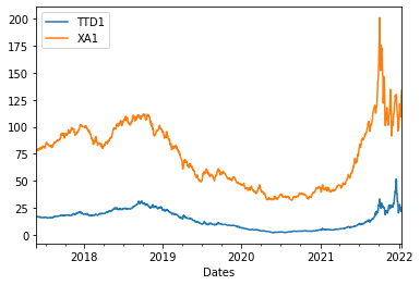
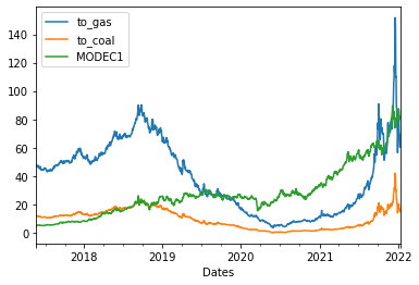
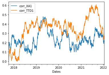
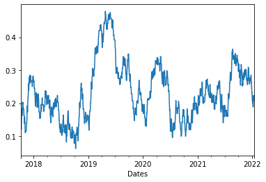
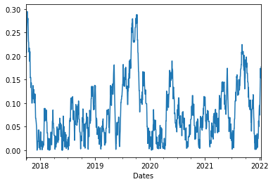
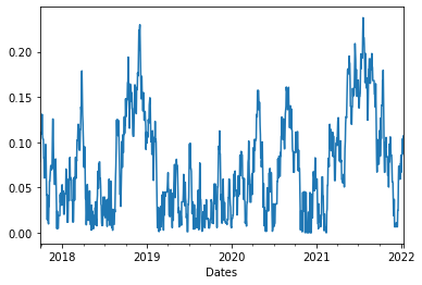
Here, I present the one with two days’ time shift. I also supply the fuel switching price and the commodities price for reference. We are curious about the magnitude of correlation, so I only present the absolute value of correlation for the below.

{width=”\textwidth”}

{width=”\textwidth”}

{width=”\textwidth”}

{width=”\textwidth”}

I found the following points that are very interesting:

• Till early 2018, the allowance price is cheap. Based on Fuel Switching Price, we just keep on using XA1. In both correlations with XA1 and TTD1, the correlation is indeed small.

• From the mid 2018 - 2020, the correlation of TTD1 and XA1 goes up.

  • From late 2018 - early 2019, we could witness the price of TTD1 is stable, but the price of XA1 had gone through bigger fluctuation. From the correlation, we could see the correlation of XA1 is indeed large and peaked, while that of TTD1 remains small.

  • From mid of 2019 to early 2020, the allowance price is between the fuel switching price. Then, the plant should switching between both fuels. TTD1 has very large corelation in that period, and indeed the price of TTD1 is going through a big decrease (decreases 70%, from 22.5 to 7). The price of XA1 is more stable in that period, hence the correlation is not as large as TTD1, but it is also larger than that in 2018. This shows the main contributor for this period is TTD1, as well.

  • In late 2020, the MODEC1 goes higher than switching price for gas, thus the allowance price is not controlled by the demand from XA1 and TTD1. We could also withness that from 2020 to the begin of 2021, the correlation is small.

• Finally, the 2021-2022 we has extreme circumstances, the price goes to peak and the correlation increase for both fuels. But I would want to stress the time of the peak of the correlation.

  • For the peak of XA1, its peak is at the third quater of 2021, and this is when XA1 is extremely high.

  • The peak of TTD1’s correlation goes to the late 2021, later than that of XA1, and it is also the time when TTD1 climbs dramatically.

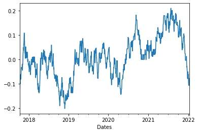
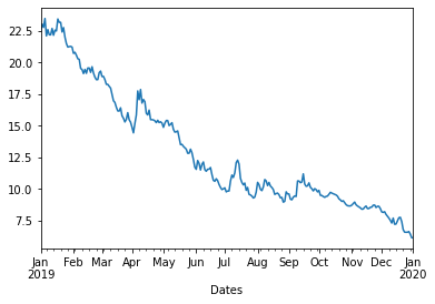
I supply a figure for the TTD1 during the year 2019, since it decrease dramatically but due to the existence of XA1 in the above figure, it is seemingly not remarkable.

{#fig:my_label width=”60%”}

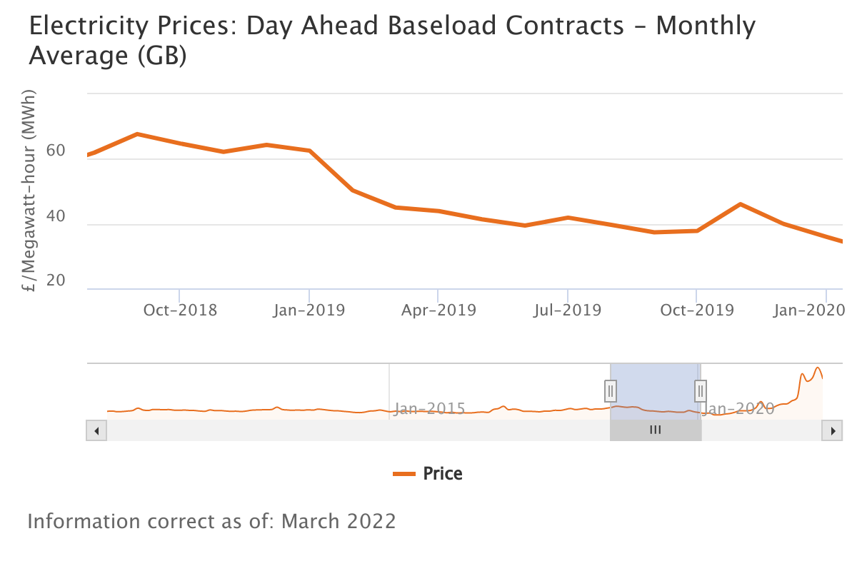
Relation with the Electricity Price

I present with the Baseload Electricity price in UK in late 2018 to year 2019 for verification.

We have the following assumption:

• Suppose the electricity is generated by the CCGT, then it is positively correlated with the fuel it uses at the time

• From the correlation analysis in the last section, we should be able to know which fuel is chosen at one stage.

Late 2018 - 2019 is a good point to analyze. Based on our assumption above, the correlation

• in late 2018 - early 2019 is high with XA1 but not with TTD1. At this period, the price of XA1 is slightly increasing and decreases, while TTD1 keeps decreasing. The electricity price is goes with the trend of XA1. This verifies our analysis that plants mainly burn XA1 and XA1 controls the price of allowance.

• from early 2019 to 2020, it is claimed in our analysis that the allowance price is controlled by TTD1 whose correlation is very high. And the price of TTD1 is decreasing stably, while the price of XA1 increases a bit from June to September 2019. The electricity price generally keeps decreasing, as is the trend of TTD1. Some one may claims the slight upward of electricity price coincides with that of XA1, but they happended in different time - the upward of electricity price is due to the approach of winter.

{width=”\textwidth”}

{width=”\textwidth”}

Due to the fact that I don’t have more access to the electricity price, I could only do this coase analysis.

Conclusion

I believe this analysis could guide the trading of Coal, Gas, Allowance and Electricity.

• This correlation analyzes when the allowance price would fluctuate

• In addition, it shows which is the main contributor for the fluctuation

• It points out the time lag phenomena. This means, we could trade allowance based on the previous fuel prices - this time gap makes the trading profitable.

• Finally, it also points out what kind of fuel the plant is based on and then guide the price dynamics of the electricity.