Introduction

EU ETS was launched in 2005 to fight global warming and is a major pillar of EU energy policy. Our aim is to trade and profit from the EU ETS and therefore, in this section, we mainly focus on mechanism and principles from the quantitative finance aspect.

Understanding the Mechanism from operating a CCGT power plant

A major impact from EU ETS to the business is on the operation of CCGT power plant. CCGT could generate power by both Natural Gas and Hard Coal. The operating cost of CCGT in one compliance period is: \(g(A, \xi) := b(\xi, \lambda(A)) + A e(\xi)\) where $b$ is the normal operating costs for fuels before imposing the EU ETS, and $A$ is the price of the carbon allowance. $\xi$ refers to the supply of electricity from this plant.

In addition, $b$ could be deemed as a convex combination of the cost from burning Gas and Coal, and $G, C$ is the cost function of generating electricity from Gas and Coal, respectively. $\lambda$ is our strategy given the allowance price is $A$.

Marginal Abatement Cost & Pricing the Allowance

Marginal Abatement Cost (MAC) impacts our strategy $\lambda$. We explain our idea for MAC as below. Suppose we want to cut down one unit of emission, our cost is: \(\mathrm{P} = \frac{\frac{G}{\eta_{gas}} - \frac{C}{\eta_{coal}}}{\frac{e_{coal}}{\eta_{coal}} - \frac{e_{gas}}{\eta_{gas}}}\) which is simplified to be: \(\mathrm{P} = \frac{\eta_{coal} G - \eta_{gas} C}{\eta_{gas}e_{coal} - \eta_{coal}e_{gas}}\) where $\eta$ is the efficiency of each fuel, and $e$ is the emission of the fuel.

Based on the trading scheme (bank and cap), suppose the Allowance Price $A$ is below $P$, we could burn more coal while buy in allowance from the market. Otherwise, we have to burn Gas and sell out the allowance on the market.

Then, suppose there is no arbitrage, we could proceed to the first theorem:

• The equilibrium allowance price equals the marginal abatement costs.

This seems trivial, but we would expand it in details for the final task in further sections.

Moreover, with regards to pricing, the mainstream is based on the following:

• Statistical Method - modelling the price process by an ARCH-GARCH process considering its seasonality and heteroscedasticity.

• Stochastic Modelling - converting the problem into a stochastic control problem - simulating $i$ participants in the market and finding the equilibrium state.

Influence and Drivers

Based on the above, we could immediately witness that key drivers for the price of EU ETS would be first of all, the price of Natural Gas and Coal.

However, for the rest market drivers, the situation differs geographically. For example, the UK market is highly mature, therefore, the price of allowance generally follows the MAC, while it is not the case in EU continent. It is argued that the price of allowance is also correlated with crude oil in some of the regions.

{#fig:oil width=”70%”}

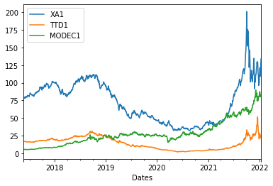
Data Specification

In this work, we are dealing with commodities futures. Due to the roll back feature, we have to do difference adjust or ratio adjust to avoid discontinuities. In this work, we use ratio adjust based on the given tickers when it comes to considering the price or PnL computation.

{#fig:my_label width=”70%”}

Correlation

One of the concern is how does the EU ETS is correlated to the other derivatives. Before we start, we have to be aware of the following two points:

• The ADF and KPSS test show that the series is likely to have unit root.

• There could be co-movements in all the commodities since they are actually correlated.

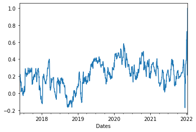
Time Varying Correlation

After taking the difference, we have the following figure for the correlation, with the rolling window of 30 days.

{width=”6cm”}

{width=”6cm”}

After reading the figure, a direct question is: Why the correlation changes all the time?

Relation with MAC / Fuel Switching Price

As is mentioned in the introduction, the Fuel Switching Price strongly impact the strategy $\lambda$. Let consider the following situation:

• The allowance price is far away from the Fuel Switching Price: This means, for small fluctuation in the price of commodities, the allowance price still remains at the same side (still greater or smaller than switching price). In other words, we are likely to maintain our strategy of which fuel to burn. Therefore, the demand of allowance remains stable - and the price of allowance would not be affected by the moves in the price of other commodities. This would imply a smaller correlation when the allowance price is far away from the fuel switching price.

• On the other hand, suppose the allowance price is very close to the Fuel Switching Price: any small fluctuation would affect the demand, and then impact the price of allowance - This implies higher correlation when the allowance price is close to the fuel switching price.

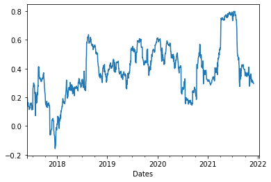
Here, we provide the curve of fuel switching price.

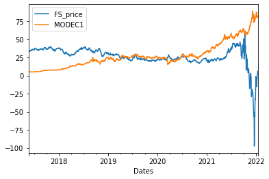{#fig:fs width=”80%”}

Let’s compare the Fig [fs]{reference-type=”ref” reference=”fs”} with the correlations. During the year 2018 to 2019, the Fuel Switching Price is off the allowance price, and as we anticipated, the correlation drops. From the year 2019 to the mid of year 2020, the Fuel Switching Price goes with the allowance price, and also we could witness the increase in correlation during the year. Finally, the beginning of year 2022 witness a diversion of the Fuel Switching Price to the allowance price, and the correlation decreases dramatically as well.

However, we could still witness some issues that the correlation is not fully connected with the distance between allowance and fuel switching price. The reasons could be:

• For the beginning part (year 2017 - 2018), there is a small increase in the correlation while the fuel switching price is not close to allowance price. This is due to the fact that we are rolling our window for computing the correlation, hence the first few observations would contain some noise.

• Another reason is that the commodities are trading in Netherlands. Netherlands’ power plant industry is not as mature as that in UK, hence, the price of allowance could still divert from the MAC.

Analysis on the BCT-USDC Data

In this part, we would first of all analyze the seasonality of the BCT data based on ARMA, SARIMAX, ARMA-GARCH models. Then we would consider enhance the out-of-sample performance. Due to the existence of unit root, we consider the differenced price and volume.

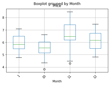
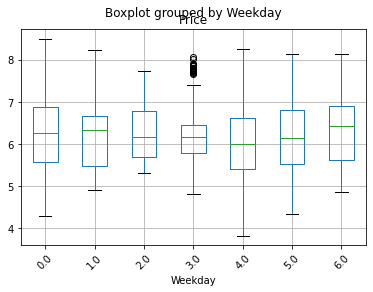
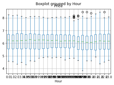
Overview of the seasonality

We group the information by the months, hours and weekdays. The following boxplot could generally give us an image of the potential existence of seasonality.

{width=”\textwidth”}

{width=”\textwidth”}

{width=”\textwidth”}

ARMA based Attempt

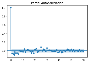
ARMA process is a combination AR and MA processes. \(\begin{aligned} \mathrm{AR(p)}: X_t &= \phi_1 X_{t-1} + \phi_2 X_{t-2} + ... + \phi_p X_{t-p} + Z_t \\ \mathrm{MR(q)}: X_t &= Z_t + \theta_1 Z_{t-1} + \theta_2 Z_{t-2} + ... + \theta_q Z_{t-q} \\ \end{aligned}\) Denoted in terms of polynomials, they are: \(\begin{aligned} \mathrm{AR(p)}: &\phi(B)X = Z \\ \mathrm{MA(q)}: &X = \theta(B) Z \\ \end{aligned}\) Where $B$ is the back-shift operator, combine them all, the ARMA process could be expressed as \(\phi(B) X = \theta(B) Z\) We look at the PACF and ACF to guess the range of the order of $p, q$.

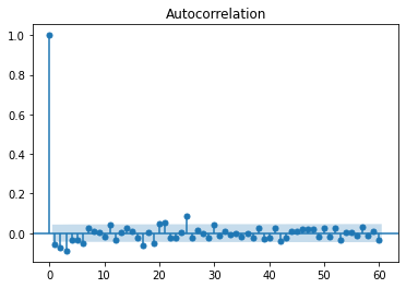{width=”6cm”}

{width=”6cm”}

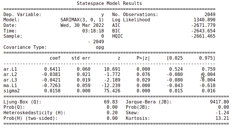
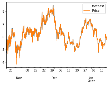
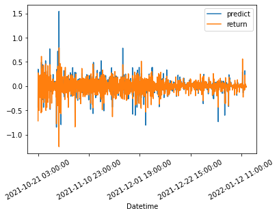
Based on the ACF, PACF, we start our search with $p < 5, q < 3$, and the best fit ARMA model is given as ARMA(3,0,1) with an AIC of $-2671.779$ (For the original data, it would be ARMA(3,1,1)). Adding the volume as the exog regressor, we would achieve the AIC of $-3044.969$. However, we would witness the problem of poor fitting.

{width=”\textwidth”}

{width=”\textwidth”}

{width=”\textwidth”}

Seasonal ARIMA model

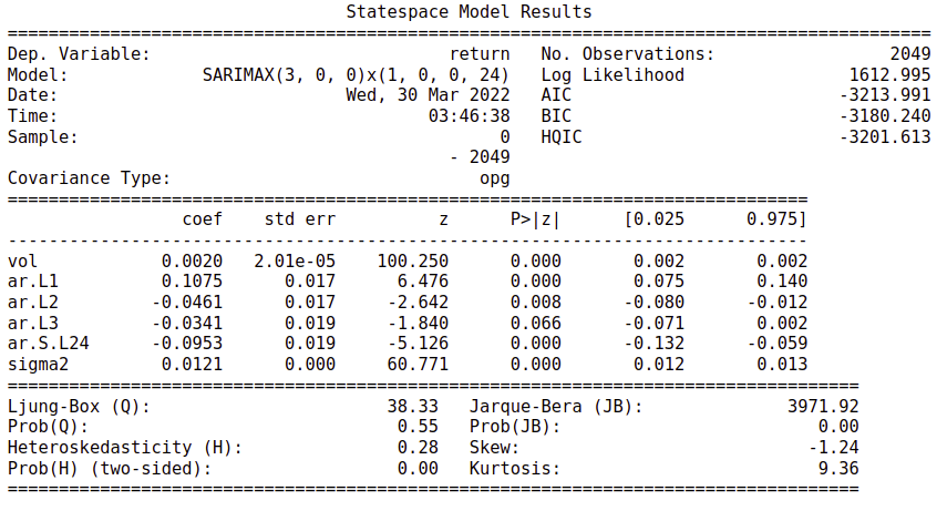
Recall the ACF and PACF figure of the return, we could witness of a correlated lag of $n = 24$. This triggers us to try the SARIMA model with the $s = 24$. This model achieves an AIC of $-3213.991$, much better than our first attempt.

{width=”\textwidth”}

{#fig:my_label width=”\textwidth”}

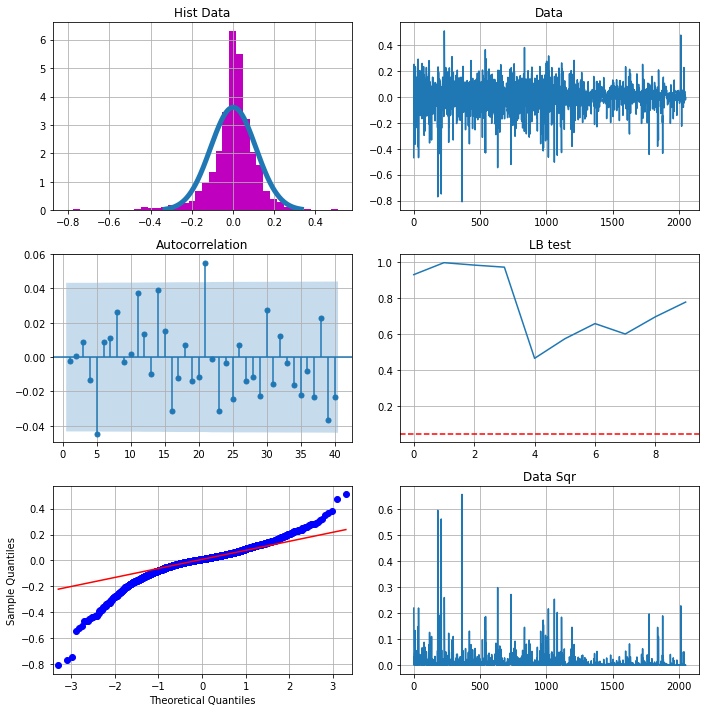
Heteroskedasticity Problem

From the diagnosis of the previous model, what we could witness is that the residuals are not white noise. They are correalted with time. This is another implication of stronger seasonality reasons that we didn’t witness.

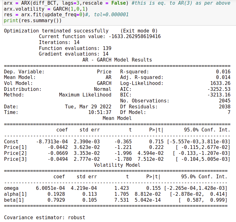
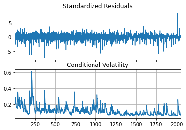
AR-GARCH approach

The general approach is to apply the AR-GARCH model. This is trivial.

{#fig:my_label width=”\textwidth”}

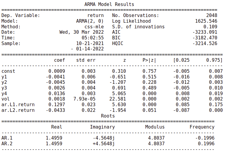
Note that, in Python we don’t have ARMA - GARCH model. We select the AR(3) since its AIC is very close to ARMA(3,0,1). We achieve an AIC to $-3252.53$.

{#fig:my_label width=”60%”}

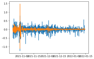
Piecewise ARIMA attempt

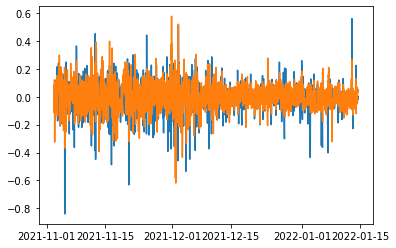
Recall the figure, we have witnessed the decreased volatility after the first period. It seems the general figure is naturally split into three stages, so is our Volume. Our idea is to slice the model into Piecewise models.

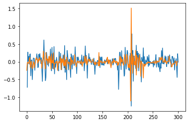{width=”\textwidth”}

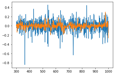{width=”\textwidth”}

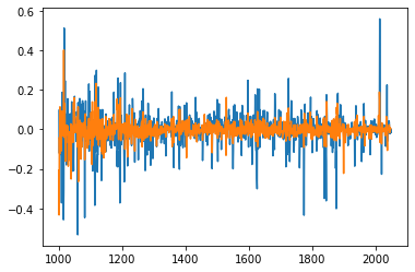{width=”\textwidth”}

Formulate the seasonality by periodic function

A problem that restricts our formulating our seasonality is the high-frequency nature of our data. Normally, the SARIMA model could only support first order model with a moderate $s$. Then, suppose our model has a monthly seasonality, it would be very hard to be captured. In addition, we can hardly capture the higher order weekly seasonality as well. A solution is to formulate the seasonality by periodic function, and use them as exog regressor. In our attempt, we tried the following approach. \(\begin{aligned} f(x) = \mathrm{sin}(2\pi \frac{x}{\omega}) \end{aligned}\) Where the $\omega$ is the periodicity. We also formulate our volume by an exponential function to reflect on the changes in volume. In our new model, we could witness an decreased AIC to $-3235.331$. In addition, we can witness the Weekday seasonality is significant.

{#fig:my_label width=”\textwidth”}

By applying a piecewise simulation, and delete the non-significant regressor, we reached the final approximation.

{width=”6cm”}

{width=”6cm”}

Out-of-sample Precision - Stochastic Control

Another problem we would curious about, is how does our model behave on the test set (overfitting). Recall what we mentioned in the first section, and here we formulate our problem to be:

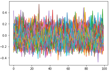
Suppose we have $N$ agents in the market and for a period of $T$. For all of them, the total fuel switching costs is given by: \(F(\lambda) = \sum\limits_{i = 1}^{N}\sum\limits_{t = 0}^{T-1} \lambda_{t}^{i} P^{i}_{t}\) And we have \(\Pi(\lambda) = \sum\limits_{i = 1}^{N}\sum\limits_{t = 0}^{T-1} \lambda_{t}^{i}\) which is the total amount of allowance we saved. We also have the overall demand for allowance as \(\Gamma = \sum \Gamma^{i}\) Therefore, the overall cost is \(G(\lambda) = -F(\lambda) - \pi(\Gamma - \Pi(\lambda))^{+}\) $\pi$ is the incompliance cost.

To further simplify the setting, we formulate the $P$ as \(\begin{aligned} P &= X(t) + L(t)\\ dX_t &= \gamma(\alpha - X(t))dt + \sigma dW_t\\ L(t) &= a + bt + f(t) \end{aligned}\) where $f(t)$ is a combination of periodic function. Then, the demand process \(\begin{aligned} \Gamma_{|t} &= Pois (\xi) \\ d\xi &= \mu dt + \sigma dB_t \\ \end{aligned}\) The function $f(t)$ is formulated by regression on basis function with the price of Natural Gas and Coal. The parameters of the Cox Process is obtained by calibrating the volume.

{width=”6cm”}

{width=”6cm”}

However, the different time frame decrease the precision.

Reference

Philipp Koenig, Modelling Correlation in Carbon and Energy Markets, Working Paper

Rene Carmona, Max Fehr, and Juri Hinz Optimal stochastic control and carbon price formation, SIAM J. Control Optim., Vol. 48, No. 4, pp. 2168-2190

Sam Howison and Daniel Schwarz Risk-Neutral Pricing of Financial Instruments in Emission Markets: A Structural Approach, SIAM Review, Vol. 57, No. 1, pp. 95-127

Sharon S. Yang, Jr-Wei Huang and Chuang-Chang Chang Detecting and modelling the jump risk of CO2 emission allowances and their impact on the valuation of option on futures contracts, Quantitative Finance, Vol. 16, No. 5, pp. 749-762

Wenlin Huang, Jin Liang and Huaying Guo Optimal Investment Timing for Carbon Emission Reduction Technology with a Jump-Diffusion Process, SIAM J. Control Optim., Vol. 59, No. 5, pp. 4024-4050