
A Parsimonious Stochastic Simulation for LOB Dynamics
The Problem
What we care about is the following: \(E(X_t | \mathcal{F}_{t-20})\) From the perspective of statistics, we are finding a regression or any other model, that characterizes the relation by learning from previous observations.
From the aspect of probability, we have a coarse mindset, that what kind of the model would be. Based on observations, we are calibrating our model parameters.
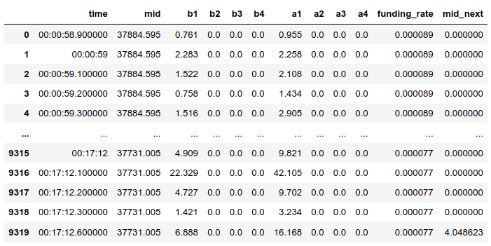
Adjustment to the data
We adjust the LOB:
Group by Time Tick
Group Bid Ask / Trade into different Classes
 {#fig:LOB}
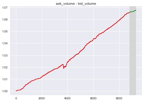
Statistical Approach - Bid-Ask Pressure
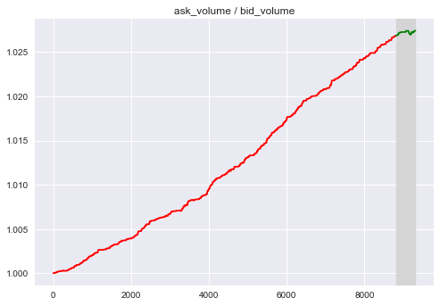
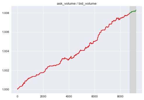
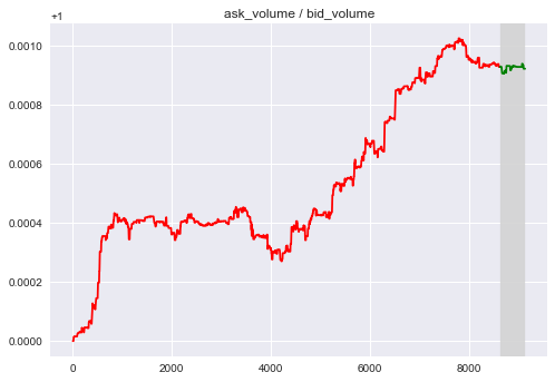
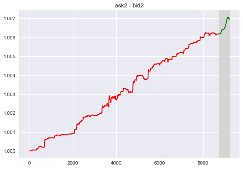
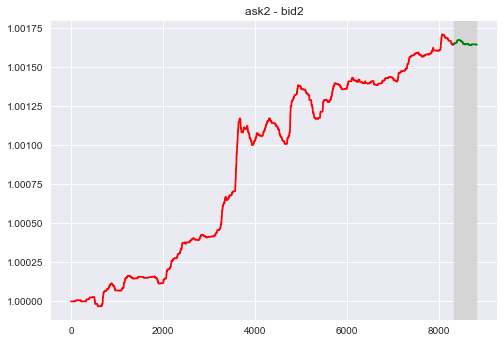
Here are two factors that is intended to reflect the pressure between buy and sell:
$F_1 = a1 - b1$ (The difference between best ask and best bid)
$F_2 = a1/b1$ (The ratio between best ask and best bid)
 {#fig:a width=”\textwidth”}
 {#fig:b width=”\textwidth”}
 {#fig:c width=”\textwidth”}
 {#fig:a width=”\textwidth”}
 {#fig:b width=”\textwidth”}
 {#fig:c width=”\textwidth”}
Both Factors have good approximation for approximate window.
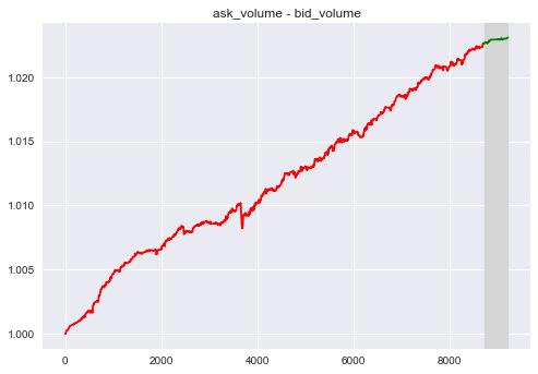
Statistical Approach - Willingness to be Executed
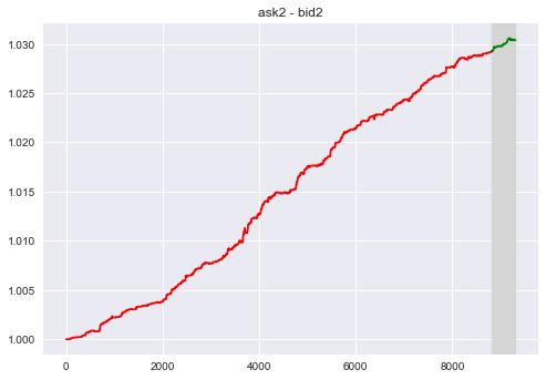
Consider the gap between the volume (price) between the second rank Bid and Ask.
- $F_3$ = a2 - b2
 {#fig:a width=”\textwidth”}
 {#fig:b width=”\textwidth”}
 {#fig:c width=”\textwidth”}
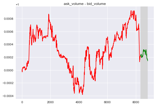
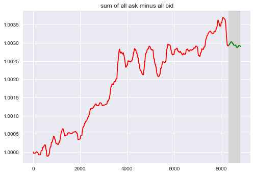
Statistical Approach - Market Situation
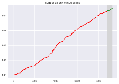
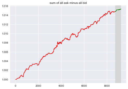
How many orders remain is also a good indicator for the market dynamics.
- $F_4 = \Sigma a_i - \Sigma b_i$
 {#fig:a width=”\textwidth”}
 {#fig:b width=”\textwidth”}
 {#fig:c width=”\textwidth”}
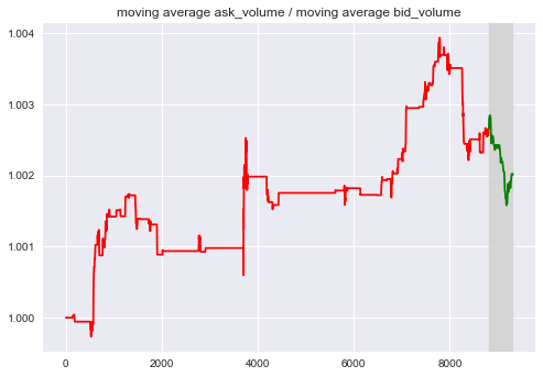
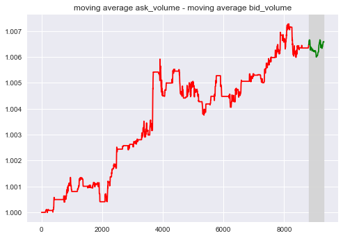
Long / Short Memory
A question is whether or not the price would be affected by the historical event that has happened long time ago? We considered the moving average of bid and ask.
 {#fig:a width=”\textwidth”}
 {#fig:b width=”\textwidth”}
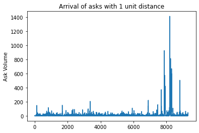
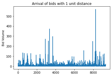
Probabilistic Approach - How many orders arrived in unit time?
The Mid Price is the average of best bid and best ask.
Poisson Process describes the arrival of events in unit time
We have to consider the randomness of the $\lambda$ and the discrete property of Poisson Distribution - Cox Process
 {#fig:a width=”\textwidth”}
 {#fig:b width=”\textwidth”}
Relation between Mid-Price and LOs
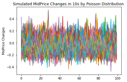
\(dS_t = (v + \alpha_t) dt + \sigma dW_t\) where \(d \alpha_t = -\xi \alpha_t dt + \sigma_{\alpha} dB_t + \epsilon^+ dL_t^+ - \epsilon^- dL_t^-\) While we simplify to the following numerical approach: \(dS_t = w \cdot dX_t\) \(X_t|_{\lambda_t} \sim Pois(\lambda_t)\) where \(d \lambda_t = \mu_t dt + \sigma_t dW_t\)
Calibrating the Model
$w$: measuring the impact of orders, OLS / WLS
$\mu$: measuring the drift of order arrivals during unit time - mean of difference
$\sigma$: measuring the volatility of order arrivals - variance of LO amount
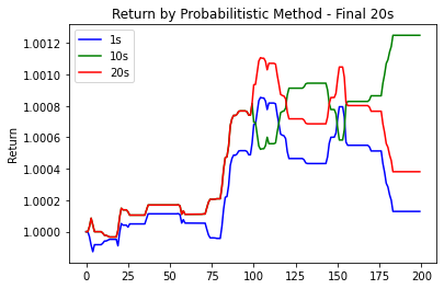
Numerical Results
 {#fig:a width=”\textwidth”}
 {#fig:b width=”\textwidth”}
Reflections on Probabilistic Model
Slow decay when the prediction interval is growing (Robustness)
Seamless connection with Optimal Execution
However, it takes longer time to run the Monte Carlo simulation